Amazon Athena and Amazon Redshift – Overview and Comparison

(Note: This is a guest post from our friends at Panoply)

Cloud-based data services are all the rage these days for many good reasons, and AWS (Amazon Web Services) is the current king of cloud-based data service providers, as this analysis carried out by StackOverflow indicates.

Two popular AWS cloud computing services for data analytics and BI are Amazon Redshift and Amazon Athena, both of which are useful for delivering actionable insights that drive better decision making from your data. However, with a dizzying amount of information available on both services, it’s a challenge to recognize what to look out for when choosing a cloud-based data service to meet your needs.

In this post, you’ll get a broad overview of cloud-based data warehousing, and you’ll come to understand the main differences between Amazon Redshift and Amazon Athena (also see this post by Panoply on the subject).

When you’re finished reading, you’ll know which service you should choose between Athena and Redshift. The comparison can also teach you what to look for in more general terms when considering any cloud-based data solution currently available.

A Data Warehouse in the Cloud

Traditional on-premise data warehouses are used for analyzing an organization’s historical data in one unified repository, pulling data from many different source systems, such as operational databases. Physical data warehouses are complex and expensive to build and maintain, though.

Cloud-based data warehouse services offer a much cheaper and easier way to use a data warehouse without needing any physical resources on site. Cloud-based providers host the necessary physical resources “in the cloud” while you simply pay for using the service.

Some examples of data warehouses in the cloud are:

  • Amazon Redshift—in Redshift, you provision resources and manage those resources similar to how you would in a traditional data warehouse, without the need to host physical computing resources on-site—AWS hosts them in the cloud instead as “clusters”. You simply connect your operational data sources to the cloud and move the data into Redshift for use with analytics and BI tools. Redshift uses a customized version of PostgreSQL.
  • Amazon Athena—Athena provides an interactive query service that makes it possible to directly analyze data stored in Amazon S3, which is the cloud storage service provided by AWS. You query data in Athena with standard ANSI SQL. In contrast to Redshift, Athena takes a serverless approach to data warehousing because you don’t need to provision resources or manage the infrastructure.
  • Google BigQuery—BigQuery is a serverless cloud-based data analytics platform that enables querying of very large read-only datasets, and it works in conjunction with Google Storage.
  • Azure SQL Data Warehouse—this Microsoft offering is a scalable and fully managed cloud-based data warehouse service.

You could write a book comparing all four of these services, so we’re going to hone in on both Amazon Redshift and Amazon Athena below.

Amazon Athena vs. Amazon Redshift – Feature Comparison

  • Initialization Time: Amazon Athena is the clear winner here because you can immediately begin querying data stored on Amazon S3. Redshift, on the other hand, requires you to prepare a cluster of computing resources and load data into the tables you create.
  • User-defined Functions: Amazon Redshift supports user-defined functions (UDFs), which are procedures that accept parameters, perform an action, and return the result of that action as a value. Amazon Athena has no support for UDFs.
  • Data Types: Amazon Athena supports more complex data types, such as arrays, maps, and structs, while Redshift has no support for such complex data types.
  • Performance: For basic table scans and small aggregations, Amazon Athena outperforms Redshift. However, for complex joins and larger aggregations, Redshift is a better option.
  • Cost: Athena’s cost is based on the amount of data scanned in each query, which means it’s important to compress and partition data. Since Amazon Athena queries data on S3, the total cost of S3 data storage combined with Athena query costs gives the full price. Redshift’s cost depends on the type of cloud instances used to build your cluster, and whether you want to pay as you use (on demand) or commit to a certain term of usage (reserved instances).


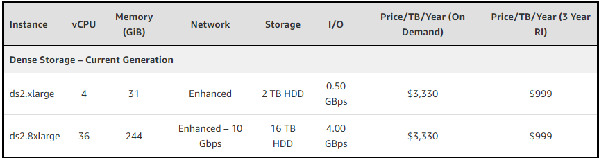
Athena’s cost is $5 per terabyte of data scanned, while Redshift’s hourly costs range from $0.250 to $4.800 per hour for a DC instance, and $0.850 to $6.800 per hour for a DS instance.

AWS Redshift Spectrum, Athena, S3

Redshift Spectrum is a powerful feature that enables data querying in Redshift directly from S3. With Spectrum you can create a read-only external table, with its data located in a specified S3 path, and immediately begin querying that data without inserting it into Redshift. You can also join the external tables with tables that already reside on Redshift.

Querying data in S3: sounds familiar, right? That’s because Amazon Athena performs a similar function—it’s an S3 querying service. It’s important to note, however, that Spectrum is not an integration between Redshift and Athena—Redshift queries the relevant data on its own from S3 without the help of Athena.

If you are already an Amazon Redshift user, it makes sense to opt for Spectrum over Athena because of the convenience. However, if you aren’t currently using Redshift, it’s best to choose Athena over Spectrum because your investment in computing resources might go underutilized in Redshift. For your current analytics needs, Athena is likely to do the job—you can always invest in a Redshift+Spectrum combination later on when it’s needed to handle lots of data.

Athena vs. Redshift – Which Should You Choose?

There is no widespread consensus on whether Amazon Athena is better than Redshift or vice versa—both services suit different uses.

  • Amazon Athena is much quicker and easier to set up than Redshift, and this querying service outperforms Redshift on all basic table scans and small aggregations. The accessibility of Athena makes it better suited to running quick ad hoc queries.
  • For complex joins, larger aggregations, and very large datasets, Redshift is better due to its computational capacity and highly scalable infrastructure.
  • The conclusion, therefore, is that Redshift is likely the cloud-based data warehouse platform of choice if you have lots of data and many complex queries to run. Amazon Athena is the recommended cloud-based service for analyzing your data in all other cases, and it’s suitable for small- to medium-sized organizations.

Closing Thoughts

Cloud-based data warehouses are quickly replacing traditional on-premise data warehouses because of their convenience, lower cost, and scalability.

Amazon Athena and Amazon Redshift take differing approaches to cloud-based data analytics services—Redshift requires resource provisioning and infrastructural management while Athena abstracts operational management away from users and allows direct querying of data stored on Amazon S3.

Amazon Spectrum provides separation of storage and compute in Redshift by allowing you to directly query data in S3, similar to Athena. Spectrum is useful if you already use Redshift, but you shouldn’t base your decision on Athena versus Redshift on the Spectrum feature.

The relevant comparison between Amazon Athena and Redshift relates to how they perform, what they cost, which tools they support, their usability, their accessibility, supported data types, and user-defined functions. You should base your end decision between Redshift and Athena on these factors, prioritizing the most important aspects of each service for your particular business. Maybe you prefer Athena’s effortless accessibility? Or maybe you’d rather the control and scalability you get in Redshift?

When weighing up any potential cloud-based data warehouse, always consider the above factors, instead of just choosing the most affordable solution.

From Academia to Industry

It has become a bi-weekly ritual. The professor spent too much time on the course material again and is left mumbling through a complex project description during the 11th hour of class. All the while, you’re off somewhere else. As you sling your backpack over your shoulder, you catch the only words you’ll need to hear: “You can download the syllabus along with the source code from the CS department’s website,” they say. Great! You hustle back to study location of choice, open your laptop, and extract the project files. After the obligatory knuckle crack, you look down at the method stubs spelled out for you. “All I have to do is fill-in these functions?” you think to yourself. And as you’re getting familiar with the project structure, a couple flicks of the scroll wheel reveal hundreds, sometimes thousands of lines of unexplained boilerplate code.

You eventually finish up the assignment and push it to the CS department’s server for grading. Without fail, someone raises their hand during the next class asking the instructor if they could explain what some of that boilerplate code was for, at which point the student is usually told to refer to the language documentation to figure it out for themselves. And for the most part, this makes perfect sense. After all, you’re there to learn about some of the more complex topics in computer science, not to write setter and getter methods all day. That’s what your data structures class was for.

But I would like to share with you the first few months of my experience as a Jr. Software Engineer and compare it to my time as an undergraduate student. You might be not-so-surprised to hear I have spent more time writing code similar to the boilerplate stuff mentioned above than I have perfecting the space and time complexity of my pioneering solution to The Traveling Salesman problem.

As an undergraduate student, I was an ace at avoiding merge conflicts in repositories where I was the only contributor. I could even run a build script with the best of ‘em. Nobody ever really told me how to use version control systems to manage a collaborative project with tens of thousands of lines of code strewn across a mess of files and directories. And if, for some reason, those same build scripts broke or a merge conflict popped up on a group project? Well, I was pretty much at the mercy of Stack Overflow.
At Setfive, when I was tasked with setting up a relational database schema for my first real project, I wasn’t really sure where to begin. There was no syllabus to refer to and no professor to schedule office hours with. While I was aware of relational database software such as MySQL and NodeJS, I had never really written a query, so I certainly didn’t know the difference between an inner and outer join. And while coordinating all those AJAX calls and setting up the Symfony bundle configs was a little confusing at first, I think I’m starting to learn how to apply my undergraduate education to these real-world projects.

So far, I have found that industry-level programming helps hone a much more practical skill set than academic programming. Don’t get me wrong, I learned a ton in college, and I know the concepts taught are not only important to a fundamental understanding of the field of computer science, but also have profound and meaningful applications elsewhere, such as in operating systems, machine learning, and so on. But when I look back on the things I have learned in such a short period of time over these past few months, it gets me excited for the road ahead. I owe an enormous thanks to Setfive for bringing me on as an entry-level software developer and advising me with patience.

JointDJ.com: Collaborative Music Tech

You might remember Txty Jukebox, our free to use collaborative music web app that we built on top of the YouTube Data API. We were happy to find that our original version was well received and even got some press from the folks over at makeuseof.com. Well, we’ve finally got a chance to spend some time ( big thanks to our new hire Josh who led the charge ) to make improvements based on the feedback we received and re-branded it under jointdj.com!

The main idea behind our music inspired web application is to create an easy way for groups of people to collaboratively share and listen to song (and video) requests. Any user with a smart phone or computer can enter the event code provided by the event’s host on jointdj.com and start submitting songs to the event’s playlist. The “event” doesn’t always have to be a traditional party either, for example, we’ve been using Joint DJ ourselves in our office as a Pandora or Spotify replacement.

To see how it works I suggest skimming the jointdj.com landing page which does a good job of quickly outlining how to use. Instead of regurgitating that information here I’ll highlight a few new features/improvements to get excited about:
  • One big lesson learned from our first go around with Txty Jukebox was that while it’s great when everyone at your event is engaged and the song queue is filled up you can run into awkward silences if the playlist runs of songs when people get distracted, say, doing work or playing an intense game of flip cup. In the past you had to wait until someone queued another song so it became a bit of a chore for the event host. To solve this issue and ensure there will never be a silent moment, we’ve created a new feature that lets the event host to pick a genre of music when they create an event from which a song will be randomly selected and played if a playlist ever runs out. For example, I could create an event with “Top 40 / Pop” as the auto fill genre. If at any point during my event the playlist is empty, all the sudden the latest Chainsmokerz song will magically be queued up!
  • Another issue we saw in the first version was that sometimes users didn’t get the exact song played that they were searching for. That was because we automatically selected the first result from Youtube regardless of whether it’s the desired result. For Joint DJ, we’ve added the ability for users to use an intuitive browser based UI to easily search for a song and then review the list of music video results from YouTube along with the thumbnail. Once the user finds exactly what song they want to play they can simply select it to add it to the event’s playlist.

  • Lastly, we improved the design of the live player view where events users can watch and listen to the music videos associated with the requests. You’ll see “flash” messages when songs are added that show the artist, title and which “DJ” submitted it. Additionally we show the next 4-5 upcoming songs in the queue along with their thumbnails on the left side of the player window. Overall, the new look is more colorful and crisp and should be more impressive to the events users keeping them engaged, having fun, and contributing songs to the event. Below is a screenshot of what the live player view looks like:

S3Grep – Searching S3 Files and Buckets

On a project we were working on recently it appeared that we had data coming into our Extract, Transform, Load (ETL) processes which should have been filtered out. In this particular case the files which we imported only would exist at max up to 7 days and on any given day we’d have tens of thousands of files that would be created and imported. This presented a difficult problem to trace down if something inside our ETL had gone awry or if we were being fed bad data. Furthermore as the files always would be deleted after importing we didn’t keep where a data point was created from.

Instead of updating our ETL process to track where a specific piece of data originated from we wanted to basically ‘grep’ the files in S3. After looking around it doesn’t look like anyone has built a “Grep for S3”, so we built one. The reason we didn’t simply download the files locally and then process them one at a time is it’d take forever to transfer, then grep each one individual sequentially. Instead we wanted to do the search in parallel and not hold the entire files on the local disk.

With this we came up with our simple S3Grep java app (a pre-built jar is located in the releases) which will search all files in a specific bucket for a specific string. It currently supports both regex or non-regex search strings. You can specify how many threads you want it to use to process the files or it by default will try to use the same number of CPU’s on your machine. It utilizes the S3 Java adapter to read the files as a stream rather than a single transfer, than read from disk. Using the tool is very simple:

A the s3grep.properties file is a config file where you setup what you are searching for. An example:

For the most part this is self explanatory. The log level will default to INFO, however if you specify DEBUG it will output some more information such as what file’s it is currently checking. The logger_pattern parameter defaults to “%d{dd MMM yyyy HH:mm:ss} [%p] %m%n” and can be any pattern you want. For more information on the formatting visit the PatternLayout Documentation.

The default output format would look something like this:

If you want a little less verbose and more of just log lines you can update the logger_pattern to be just %m%n and end up with something similar to:

The format of the output is FILE:LINE_NUMBER:matching_string.

Anyways hope this helps you if you are trying to hunt down what file contains a text string in your S3 buckets. Let us know if you have any questions or if we can help!

Symfony2 – Moving to Translatable Entities

In my last post I talked about setting up Symfony2 entities for translation and integrating it with Sonata Admin. One of the trickier parts of moving from a non-translatable entity to a translatable one is the migration of your data.

To understand some of the complexities with the migration you must understand the changes to the database that occur when taking an entity from being a regular entity to a translatable one. Any columns that are translatable will now live on a separate table and the old column is no longer used. Let’s use the following pre-translation entity DB schema as an example:

For this entity we’ll make visible_label translatable, following the instructions in my previous post. This will result in the following final schema:

The column “visible_label” has moved from the regular entity table to the entity’s translation table. If you had data in the visible_label previously it would be lost as that column no longer exists. Since we had tons of data in our case this wasn’t acceptable.

To make sure we didn’t lose data, we did the translatable migration in two stages. First, we kept the columns we were translating in the original entity and only removed the getters and setters. The reason we removed the getter and setters is we wanted to utilize the magic __call() method so it would return values from the translatable entity. All that was left was the original column declaration. At first it seemed like making the column variable public for the time being would be a quick and easy solution, then run a script that reads the public variable and migrates it to the translation. The problem with this approach is Twig will read out the public variable rather than calling through the __call() method to the translatable entity. Since we were testing at the same time as trying to build the migration, we needed the tests to access the translatable entity and not the old public variable. We ended up using Reflection Classes and keeping the column declared as a private. With reflection you can change properties to be accessible outside of the class even though they are declared private. For example:

By using the reflection we’re able to access the original “visible_label” column and migrate the data to the translation entity. We built similar routines for each of the entities that we had to migrate. After the migration and everyone confirmed that the live site was functioning properly, we removed the translated columns from the original entity and database.

By taking this two staged approach we were able to move to translatable entities while not losing any data in the migration. In our case we also marked (//START TRANS, //END TRANS) on each entity the start of translatable columns and end so that we could use sed to go through all of them and remove the old columns once the migration was finished.

Happy translating!